Tech art for art directors

I see that the slides from my 2015 GDC talk, Technical Art For Art Directors is now up on the GDC Vault. paywall warning Enjoy – and feedback in the comments is very welcome. I can post the slides if there is interest, but if you watch the video you’ll see that they don’t really work without the verbal context. I defy anybody who wasn't there to make sense of this image, for example....

I’ll say in passing that – despite the lack of text in the finished presentation – I had great luck putting this talk together in Markdown using DeckSet, which let me do the first 90% of the presentation without ever opening PowerPoint or Keynote. The slides were just one big plain text file, which let me put them up on github so I could version them and track changes without getting bogged down in the finicky formatting nonsense that ultimately consumes all slide decks. I particularly liked this workflow because I could work as if it was text but still run it as a slide show very early on, which gave me a chance to get my patter down and listen to the words instead of getting hung up on formatting text. Plain text FTW!

Book Review

Computer books are a very hit-or-miss affair. I go through them like comic books but – like comic books – they rarely have much of an impact on me: I read along, nod, and ten minutes after I close the covers I’ve either compressed the whole thing into a crunched-down, dried-up mental summary or filed it away as something to look at for a very specific kind of reference.
It’s hard for a technical book to really engage a reader. Clarity, clean exposition and simply not peddling misinformation by accident or oversight are hard enough and many tech books fail to even hit those mares. Engaging style and memorable insights are even tougher to conjure up.

My personal favorite in this regard is The Art Of Readable Code by Dustin Boswell and Trevor Foucher. Unlike most tech books it’s not about technology, it’s about you. By which I mean it’s about how to approach programming problems with a pragmatic, long term view that’s about making your life more productive and less stressful in the long run by adopting smart practices. It’s not about whiz-bang tech - in fact, the book hops around between languages and problem sets and doesn’t really teach anything about programming per se; rather, it’s about writing: about making your code clear, expressive and humane. Programmer machismo often encourages us to write super-efficient alien artifacts which can be extremely impressive but which nobody wants to touch for fear of getting the Space Odyssey treatment. I’ve started forcing this book on all my new people: it’s better than a style guide because it teaches you things to think about, rather than giving you a list of things to memorize and follow.
(hat tip to @Pat Corwin, by the way, who turned me on to this one)
What got me thinking about tech books just now is the fact that I’ve recently found one that’s almost but not quite in that elite class of game changers. Effective Python, by Brett Slatkin, is more technical and a bit less fluent than The Art Of Readable Code. Still, it caught my eye because it seems like a great mile-marker on the road from “pretty good python user” to “real Pythonista.”

Effective Python does a great job of explaining and illustrating several features of the language which can be overlooked by folks coming from a scripting background rather than computer science. Many of the habits which separate the Python zen masters from the mere acolytes are explained neatly and clearly: the mysteries of the yield keyword, the evils of the mutable default argument, and the unfathomable allure of metaclasses are all dealt with clearly and in ways that don’t make you feel like a chump. Even better, the information is presented with a usable, practical slant: it’s neither an abstract set of rules to memorize nor a comp-sci nerdout about language features. Instead the book presents enough information for you to make good strategic choices: Perennial python puyzzlers like “list comprehension or loop?”, “Is it okay to use Try…except…else?” and “When to use propertites vs descriptors vs plain old fields” are all addressed in a reasonable, non-dogmatic way.
So, I’ll definitely be adding that one to the new-hire reading list in the future. Recommended!
PS if you haven’t checked out the Tech Art Bookstore in a while, I’ve added a bunch of new items over the last few months

Goddamit, stop messing around

It was inevitable, after I started noodling around with terminal colors in ConEmu, that I’d waste an afternoon cooking up a way to color my Maya terminal sessions automatically.
The actual code is up on GitHub (under the usual MIT Open License - enjoy!).

As implemented, its a module you can activate simply by importing conemu. Ordinarily I don't like modules that 'do things' on import, but this one is such a special case that it seems justifiable. Importing the module will replace sys.stdout, sys.stdin, and sys.display_hook with ConEmu-specific classes that do a little color formatting to make it easier to work in mayapy.  If for some reason you want to disable it, calling conemu.unset_terminal() will restore the default terminal.

Here are the main features:

Colored prompts and printouts

This helps de-emphasize the prompt, which is the least interesting but item on screen, and to emphasize command results or printouts

Unicode objects highlighted

Since all Maya objects returned by commands are printed as unicode string (like u'pCube1', the terminal highlights unicode strings in a different color to make it easy to pick out Maya objects in return values. The annoying little u is also suppressed.

Code objects highlighted

Code objects (classes, functions and so on) are highlighted separately

Comment colors

Lines beginning with a # or a / will be highlighted differently, allowing you separate out ordinary command results from warnings and infos. In this version I have not isolated the path used by cmds.warning, which makes this less useful. Does anybody out there know which pipe that uses? It appears to bypass sys.stdout.write() and sys.stderr.write()

Automatic prettyprint

If the result of a command is anything other than a string, it will be run through prettyprint so that it will be formatted in a slightly more legible manner. This is particularly handy for commands like ls or listAttr which produce a lot of results: pprint will arrange these vertically if they result would otherwise be wider than 80 characters.

Utilities

The module contains some helper classes if you want to make your own display more elaborate, or to mess with it interactively during a console session.

Terminal: screen formatting

The Terminal class makes it less cumbersome to control the display. The main use is to color or highlight text. The 16 terminal colors are available as Terminal.color[0] through Terminal.color[15], and you can highlight a piece of text like so:

print "this is " + Terminal.color[10]("colored text")

The background colors are Terminal.bg[0] through terminal.bg[5] and work the same way:

print Terminal.bg[2]("backgound text")

Terminal also has a helper for setting, coloring, and unsetting prompt strings.

Conemu: console control

The Conemu class includes some limited access to the more elaborate functions offered by ConEmu (The methods in Terminal might work in other ANSI terminals – I haven’t tried ! – but the ConEmu ones specific to ConEmu). The key methods are:

ConEmu.alert(message)

Pops up a GUI confirm dialog with ‘message’ in it.

ConEmu.set_tab(message)

Sets the name of the current ConEmu tab to ‘message’.

ConEmu.set_title(message)

Sets the name of the current ConEmu window to ‘message’.

ConEmu.progress(active, progress)

if active is True, draw a progress indicator in the window task bar at progress percent. For example ConEmu.progress(True, 50) overlays a 50% progress bar on the ConEmu task bar icon. If active is false, the progress bar is hidden. This can be handy for long running batch items

The right profile

Lately I was working in one of those relatively rare TA tasks where performance really mattered. I had to do a lot of geometry processing and the whole thing was as slow as molasses, despite all my best guesses about clever little tricks to speed things up.

To break the logjam, I resorted to actual profiling, something I tend to avoid except in emergencies.

Now, you might wonder why I say I avoid profiling. If you skip ahead and see the trick I used here, and all the fiddly little bits of detailed performance data it provides, you may be particularly curious why anybody would want to pass up on all this cool, authoritative data. The reason, however, is really simple: Good profiling is so powerful that it can be overly seductive. Once you can see right down to the millisecond how tiny tweaks affect your code, the temptation to start re-working everything to shave a little bit off here and there is hard to escape.

If you’re working on a game engine, constant reference to the profiler might make sense. In regular TA work, however, milliseconds rarely matter: all that counts is the user’s perception of responsiveness. Your users will care about the difference between a .1 second tool and a 1 second tool, or that between a 1 second tool and a 10 second tool. They are unlikely to care about – or even notice – the difference between a 1.3 second tool and a 1.1 second tool. The time you spend grinding out those extra fractions of a second may just not be worth it. As Donald Knuth, one of the great-grandaddies of all programming put it:

We should forget about small efficiencies, say about 97% of the time: premature optimization is the root of all evil.

So a word of warning before we proceed. Optimize late, only after you’ve got the problem solved and after you’ve got what seems like solid, working code that’s just too slow. Stay focused on clarity, reliability and ease of maintenance first; only reach for the profiler in code where the perf has really become an issue.

Cheap-ass profiling

Python includes some excellent native profiling tools. The easiest one to use (and the one that’s most handy for people working in Maya) is the cProfile module. It allows you to extract very detailed timing and call-count information from a run of a function.

Here’s a basic example of profile in action. We’ll start of with a couple of simple functions.

import time
import cProfile


def some_math(n):
    return n ** n

def slow():
    time.sleep(.01)

def do():
    counter = 0
    for i in range(200):
        counter += 1
        some_math(counter)
        slow()

Then we’ll call them using cProfile.run(). The run function takes a string which it will use eval to execute. So in our case:

cProfile.run('do()')

That will print out the following report, or something pretty like it:

     604 function calls in 2.096 seconds

Ordered by: standard name

ncalls  tottime  percall  cumtime  percall filename:lineno(function)
    1    0.002    0.002    2.096    2.096 <maya console>:12(do)
  200    0.003    0.000    0.003    0.000 <maya console>:6(some_math)
  200    0.002    0.000    2.091    0.010 <maya console>:9(slow)
    1    0.000    0.000    2.096    2.096 <string>:1(<module>)
    1    0.000    0.000    0.000    0.000 {method 'disable' of '_lsprof.Profiler' objects}
    1    0.000    0.000    0.000    0.000 {range}
  200    2.089    0.010    2.089    0.010 {time.sleep}

The first line in the report prints out the total time, in this case a shade over 2 seconds. Each line in the report that follows lists the following information for a single function call (including nested calls)

ncalls

The number of times a given function was called during this run. If the function is recursive, this number may show up as two numbers separated by a a slash, where the first is the true number of total calls and second the number of direct, non-recursive calls. As you can see here do() itself was called only once, but the sub-functions some_math() and slow() were each called 200 times; time.sleep() was called 200 times as well since it was called by every iteration of slow()

tottime

the total amount of time spent executing this function for the entire run. As you can see the call to time.sleep occupies the bulk of the time in this run. Not that this is the time it takes to process the function – not the real-world time it takes to run! So our do() function in the first line shows a tottime of .002 seconds even though it clearly took more than two seconds to run.

percall

The average time spent executing the function on this line, if it was executed multiple times. Like tottime, this measures processor time only and does not include things like network delays or (as in this case) thread sleeps.

cumtime

this is the real world time needed to complete the call, or more precisely the total real world time spent on all of the calls (as you can see, it’s the sleep call and do() which each take up about two seconds)

percall

the second percall column is the amount of average amount of real-world time spent executing the function on this line.

filename

this identifies the function and if possible the origin of the file where the function came from. Functions that originate in C or other extension modules will show up in curly braces.

As you can see this is incredibly powerful right out of the box: it lets you see the relative importance of different functions to your overall perfomance and it effortlessly includes useful back-tracking information so you can find the offenders.

Record Keeping

If you want to keep a longer term record, you can dump the results of cProfile.run() to disk. In this form:

cProfile.run('do()', "C:/do_stats.prf")

You’ll get a dump of the performance data to disk instead of an on-screen printout. A minor irritant is the fact that the dumped stats are not the plain-text version of what you see when running the stats interactively: they are the pickled version of a Stats object: just opened in a text editor they are gibberish.

To read them you need to import the pstats module and create a new Stats from the saved file. It’s easy:

import pstats
disk_stats = pstats.Stats("C:/do_stats.prf")

Calling the print_stats method of your new Stats object will print out the familiar report. You can also use the sort_stats method on the object to reorganize the results (by call count, say, or cumulative time).

The details on the Stats object are in the docs

Caveats

I’ve already said that this kind of information can tempt you to cruise past to point of diminishing returns right on to squeezing-blood-from-a-stone-land. That said it’s also worth noting that there is also bit of the Heisenberg uncertainty principle at work here: profiling slightly changes the performance characteristics of your code Game engine programmers or people who do embedded systems for guided missiles will care about that: you probably don’t need to.

In any case, approaching this kind of profiling with the wrong mindset will drive you crazy as you chase micro-second scale will-o-the-wisps. The numbers give a good general insight into the way your code is working, but don’t accord them any larger importance just because they seem seem so official and computer-y. They are guidelines, not gospel.

Using the data

When you actually do start optimizing, what do you want to do with all those swanky numbers? The art of optimizing code is waaaay too deep to cover in a few paragraphs but there are a couple of rules of thumb that are handy to think about while learning how to read the profile results:

Call Counts Count

The first thing to look at is not the times: it’s the call counts.

If they seem wildly out of line, you may have inadvertently done something like call a more than you intended. If you have a script that does something to 500-vertex object but a particular vertex-oriented function shows up 2000 or 4000 times, that may mean you’re approaching the data in an inefficient way. If it becomes something huge – like 250,000 calls – it sounds like you’re doing an “all against all” or “n-squared” check: an algorithm that has to consider not just every vert, but every vertex-to-vertex relationship. These are generally something to avoid where possible, and the call count totals are a good way to spot cases where you’ve let one slip in by accident.

The evils of ‘n-squared’ and so on are illustrated nicely here. You might also want to check out Python Algorithms if you’re really getting in to waters where this kind of thing matters!

Look for fat loops

The second thing too look at is the balance of times and call counts. The most performant code is a mix of infrequent big calls and high-frequency cheap ones. If your stats show a high call count and a high cumtime on the same line, that’s a big red flag saying “investigate me!” As you can see in the report above, the real villains (slow() and in turn time.sleep()) are easily spotted by the combination of high call counts and high cumtime numbers.

Use builtins where possible

Next, you want to check the balance between your own code and built-ins or Maya API code, as indicated by the curly brackets around the function names in the last column. In general, API or built-in calls are going to be faster than anything you write yourself: doing things like a deriving the distance between two 3-D points will usually run about 8x faster in the API than it would in pure python. So, you’d like to see lots of those kinds of calls, particularly inside loops with high call counts.

High cumtimes

Only after you’ve sorted through the high call counts, and high call/cumtime combinations, and aggressive use of builtins do you want to start looking at high cumtimes on their own. Of course, you won’t have a good idea when those high times are justified if you don’t know how the code actually works, which is why you want to do your optimizing passes on code that is already legible and well organized.

Wrap

Naturally, these few notes just scratch the surface of how you optimize – this post is really about profiling rather than optimizing. I’m sure we’ll hit that topinc some other day. In the meantime, it’s worth spending some time mastering the slightly retro, programmer-esque interface of the cProfile module. Doug Hellman’s Python Module Of the Week article on profiling is a good if you want to get beyond the basic report i’m using here. There’s also a nice lightweight intro at Mouse vs Python. The docs could be more friendly but they are authoritative.

In the meantime, readers of a certain age will certainly remember who really had the right profile

Didn't need those eyeballs anyway!

OK, I admit this one is pretty much useless. But it’s still kind of cool :)
Just the other day I discussed setting up ConEmu for use as a direct maya terminal. This is fun, but once you’ve got the console virus the next thing that happens is you start getting obsessed with stupid terminal formatting tricks. It’s almost as if going text modes sends you past the furthest apogee of spartan simplicity and starts you orbiting inevitably back towards GUI bells and whistles.
At least, I know that about 15 minutes after I posted that last one, I was trying to figure out how to get colored text into my maya terminal window.
It turns out it’s pretty easy. ConEmu supports ANSI escape codes, those crazy 1970’s throwbacks that all the VIM kiddies use on their linux machines to make ugly termina color schemes:

all this beauty... in your hands!

This means any string that gets printed to ConEmu’s screen, if it contains color codes, will be in color! You can change background colors, foreground colors, even add bold, dim or (God help us) blinking text to your printouts.
Here’s a quick way to test this out:
Start up a maya command shell in ConEmu (instructions here if you missed them last time).
In your maya session, try this:

import sys
sys.ps1 = "Maya> "

This swaps in the custom prompt Maya> for the generic >>>.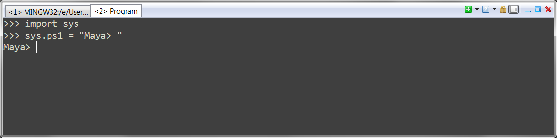

Now, let’s try to make it a bit cooler: try setting sys.sp1 to this:

sys.ps1 = "\033[38;5;2mMaya>\033[0m "

Whoa!
Here’s what the gobbledygook means:
\033 is the ascii code for ‘escape’, which terminals use to indicate a non-printable character. The square bracket - number - m sequences are displayc ommands which will affect the output. In this case we said “set the text mode to color index 2’ (probably green on your system), type out ‘Maya> ‘, then revert to the default color”.
Here’s a few of the formatting codes that ConEmu supports:

• \033[0m resets all escapes and reverts to plain text.
• \033[1m and \033[2m start or end bold text
• \033[4m turns on ‘inverse’ mode, with foreground and background colors reversed
• \033[2J clears the terminal screen and sets the prompt and cursor back to the top. You probably don’t want to use this as your prompt, since it clears the screen after every key press! However it can be useful for paging through long results, Unix-more style.
• 033[38;5;<index>m sets the text color to the color <index>. Colors are defined in the ConEmu settings dialog (Features > Colors). There are 16 color; here you identify them by index number (Color #0 is the default background, color #15 is the default foreground) This allows you to swap schemes – several well known codiing color schemes such as Zeburn and Solarized are included in ConEmu.
• 033[48;5;<index>m sets the background color to the color <index>. The background colors are a bit hard to spot: if you check the colors dialog you’ll see a few items have two numbers next to them (such as ‘1/4’ or ‘3/5’). The second number is the background index. Yes, it’s wierd – it was the 70’s. What do you expect?
• \033[39m resets any color settings.

These codes work sort of like HTML tags; if you “open” one and don’t “close” it you’ll find it stays on, so while you’re experimenting you’ll probably experience a few odd color moments.
But still… how cool is that? Now if we could only get it to syntax highlight… or recognize maya objects in return values… hmm. Things to think about :)
The Full list of escape codes supported by ConEmu is here

Con Job

If you do a lot of tools work in maya – particularly if you’re working one something that integrates with a whole studio toolset, instead of being a one-off script – you spend a lot of time restarting. I think I know every pixel of the last five Maya splash screens by heart at this point. A good knowledge of the python reload() command can ease the pain a bit, but there are still a lot of times when you want to get in and out quickly and waiting for the GUI to spin up can be a real drag.
If this drives you nuts, mayapy - the python interpreter that comes with Maya - can be a huge time saver. There are a lot of cases where you can fire off a mayapy and run a few lines of code just to validate that things are working and you don’t need to watch as all the GUI widgets draw in. This is particularly handy if you do a lot of tools work or script development, but’s also a great environment for doing quickie batch work – opening a bunch of files to troll for out of date rigs, missing textures, and similar annoyances.
All that said, the default mayapy experience is a bit too old-school if you’re running on Windows, where the python shell runs inside the horrendous CMD prompt, the same one that makes using DOS so unpleasant. If you’re used to a nice IDE like PyCharm or a swanky text editor like Sublime, the ugly fonts, the monochrome dullness, and above all the antediluvian lack of cut and paste are pretty offputting.
However, it’s not too hard to put a much more pleasant face on mayapy and make it a really useful tool.

Maya Bug Watch: API2 and GetPoints()

In general I’m more or less a fan of Maya Python API 2.0. It’s more pythonic and feels faster than the old version. However, it’s not without its quirks and I just found one that really bit me in the behind.
If you want to get the vertices of an object in the api, the usual formula is:

1. Get the dagPath of the object
2. make an MFnMesh
3. call the ‘GetPoints’ method of your mesh
4. party on.

Something like this, which returns a list of MPoint objects for the verts in the mesh

import maya.api.OpenMaya as api

def get_verts(mesh):
    mobj = api.MGlobal.getSelectionListByName(mesh).getDagPath(0)
    # that's lazy, it assumes that the first child is the mesh shape.
    # in practice you need to be more careful...
    mfn_mesh =  api.MFnMesh(mobj)
    vert_array = mfn_mesh.getPoints()
    return [i for i in vert_array]

This works fine and dandy… except:
If the mesh has 256 or more verts, the first vertex comes back as garbage
Here’s an example, using the same function:

mesh, _ = cmds.polyCube(sw = 1, sh= 1, sd = 1)
print get_verts(mesh)[:4]
#> [maya.api.OpenMaya.MPoint(-0.50000000000009082, -0.5, 0.5, 1), maya.api.OpenMaya.MPoint(0.5, -0.5, 0.5, 1), maya.api.OpenMaya.MPoint(-0.5, 0.5, 0.5, 1), maya.api.OpenMaya.MPoint(0.5, 0.5, 0.5, 1)]

# this looks good... Here's the same thing for a 226 vert cube:
mesh, _ = cmds.polyCube(sw = 8, sh= 8, sd = 3)
print get_verts(mesh)[:4]
#> [maya.api.OpenMaya.MPoint(-0.50000000000005185, -0.5, 0.5, 1), maya.api.OpenMaya.MPoint(-0.375, -0.5, 0.5, 1), maya.api.OpenMaya.MPoint(-0.25, -0.5, 0.5, 1), maya.api.OpenMaya.MPoint(-0.125, -0.5, 0.5, 1)]

# but up the vert count to 258:
mesh, _ = cmds.polyCube(sw = 8, sh= 8, sd = 4)
print get_verts(mesh)[:4]
#> [maya.api.OpenMaya.MPoint(5.0277956463997711e-315, 5.0313386899592279e-315, 0.5, 1), maya.api.OpenMaya.MPoint(-0.375, -0.5, 0.5, 1), maya.api.OpenMaya.MPoint(-0.25, -0.5, 0.5, 1), maya.api.OpenMaya.MPoint(-0.125, -0.5, 0.5, 1)]

# that first point is gibberish: python can't go to the -315th power!

I’ll leave it to wiser heads to figure out why it works out like this. My guess is that something is borked in pointer math going on inside the wrapper around MfnMesh, but I don’t know. Luckily, there’s a workaround: if you create new MPoints out of the items coming back from the GetPoints() call, you get good data. I’m not sure why but this should be so but it appears to be reliable on my machine (Windows 7, 64 bit maya 2015). Here’s the workaround:

def safe_get_verts(mesh):
    mobj = api.MGlobal.getSelectionListByName(mesh).getDagPath(0)
    mfn_mesh =  api.MFnMesh(mobj)
    vert_array = mfn_mesh.getPoints()
    return [api.MPoint(i) for i in vert_array]  # creating new MPoints fixes the issue

mesh, _ = cmds.polyCube(sw = 10, sh= 10, sd = 10)
print safe_get_verts(mesh)[:4]
#> [maya.api.OpenMaya.MPoint(-0.5, -0.5, 0.5, 1), maya.api.OpenMaya.MPoint(-0.40000000596046448, -0.5, 0.5, 1), maya.api.OpenMaya.MPoint(-0.30000001192092896, -0.5, 0.5, 1), maya.api.OpenMaya.MPoint(-0.20000001788139343, -0.5, 0.5, 1)]