 |
| There was a time when this was 'computer graphics' |
Once you start looking closely, you'/ll find that dot product and a matrix actually have a lot in common. As an older gentleman once told me when I proudly showed hin a 72 dpi dithered picture printed on my 1986 vintage Apple 2, "Wait a minute... it's all just.... dots?"
In fact, matrix multiplication is done by using dot products, as we’ll see shortly. However, matrices are more complicated, both in concept and execution. For that reason we'll devote this post through how matrices work in the simplest possible way, so that it’s easy to see both the how and why of what they do. This post will be primarily about the most minimal example of how a matrix functions. I’ll do it in 2-d to keep the math a bit less wordy, though the same thing works in 3 or even more dimensions. I’ll also be sticking to a simple rotate-only matrix to start with so the workings are simple - I’ll add in translations and scales next time out to keep the focus on the basics.
First things first
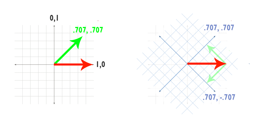
So, starting with the bare minimum, let’s suppose we've got a simple unit-length vector
[1,0] and we’d like to figure out how to rotate it. Rotating that unit vector 45 degrees should end up as [.707, .707], as you can see below: |
| We're trying to figure out an operation that will give these values as we rotate from [1,0] to [0,1] |
The question is, what kind of operations do we need to do to perform that rotation? What tools do we have to make it work - and, even more importantly, to make it work for any vector and not just this one example?
First, just to clear the decks, let's check off things we know wont’ work.
We can see that difference between the first vector and the second is
[-.293, .707] – but it’s pretty obvious that simple addition is not the same thing as performing a rotation. If you’re not convinced, just note that adding the same vector again will get you [.121, 1.414] rather than the expected [0,1]. Plain old multiplication either - there is no number we can multiply against the original
[1,0] that will get a non-zero result in the Y component.So what can we do? Fortunately, our old friend the dot product comes to the rescue. If you recall how we introduced dots, you should remember that one of the uses of the dot product is to project one vector on to another.

So suppose what would happen if we tried to project our first vector onto another vector that looked like a rotated coordinate system. In other words, we could hold our original vector constant and ‘rotate’ the X-axis counterclockwise by 45 degrees. It’s a theory-of-relativity kind of thing: rotating our vector N degrees clockwise and rotating the world N degrees counter-clockwise are the same thing. By projecting our X-axis against the rotated vector, though, we get the X component we want from a 45 degree angle.
 |
| rotating a vector (left) is the same as counter-rotating the coordinate system (right) |
We can use the unit circle (or the chart of angle values above) to figure out what the right vector for the counter rotated X-axis is. In the rotated-X-axis world we will be dotting
[1,0] against the vector [.707, -.707]:dot ([1,0], [.707, -.707])
equals
(1 * .707) + (0 * -.707) = .707
That operation gives us a good X-component - it represents how much of the original X is left when projected onto an X axis that has been rotated. If we do it again - remember, we’re trying to get a repeatable operation - we get
dot ([.707, .707], [.707, -.707])
equals
(.707 * .707) + (.707 * -.707) = 0
Which is what we want for the X component after two rotations. This dot product thing seems to be paying off (and I should know – I’ve been milking it for posts for a while).
Of course, this only gives us half of the rotated vector! However, analogy suggests that we can get the Y component of the vector by projecting onto a rotated Y axis, just as we did for the X. The Y axis, rotated clockwise 45 degrees, is
[.707, .707]. Dotting against our original vector gives usdot ([1,0], [.707, .707])
in other words
(1 * .707) + (0 * .707) = .707
which is the Y component we want after one application. The same operation on the rotated vector gives us
dot ([.707, .707], [.707, .707])
namely
(.707 * .707) + (.707 * .707) = 1
Again, this gives us the Y value we expect for a 90 degree rotation.
 |
| An example matrix showing a 90 degree rotation |
Dots to Matrix
So, that shows we can rotate a vector by using two dot products: dot the X component of the vector against a counter-rotated X axis and the Y component of the vector against a counter-rotated Y axis, and you get the rotated result. (Remember, the axes are rotated against the rotation you’re actually applying, because you want the projection of the rotated vector and you’re moving the universe instead of the data, Einstein-style).Now that we know how it works, it would be nice to have a simple way of saying “just do that two-dot thing” - in other words, we'd like to define an operation that will apply the two dot products at the same time, giving us the rotation we're after. And that’s all that the matrix - the mysterious whatchamacallit at the heart of 3-D math – really boils down to this: it’s simply a convention for saying “make a new vector out of these dot products”.
 |
| I kind of hate the internet... but I must admit, the mere existence of a pepakura Minecraft character for Dot Matrix from Spaceballs warms my heart. |
[1,0] * [  .707,  .707]
        [ -.707,  .707]
Where the first column of the matrix is the X-axis of our counter-rotated coordinate system and the second column is the Y-axis of the same. It's just a convention for saying:
x = [1,0] dot [ .707, -.707]
y = [1,0] dot [ .707,  .707]
which is exactly the same thing we took a couple of paragraphs above to explain in words.
So in the end it’s amazingly – almost embarrassingly – simple: you dot your vector against each of the columns in the matrix in turn and voila! you’ve got a new vector which applies the matrix transform. The big, scary matrix monster turns out not to be so scary - once you pull off this mask it turns out to be nothing but Old Man Dot Product in disguise!
 |
| It would have worked, too, if it wasn't for you meddling kids! |
The big takeaway from this exercise is that the basic math is the same and it requires no skills you didn’t learn by seventh grade (or at least the first post in this series). Matrices just aren't that hard once you know what they are actually doing.
As I've said several times, all of this power is really based on simple math (addition and multiplication) disciplined by conventions such as normalized vectors in dot products or the row-column arrangement I’ve shown here. A convention, however, is to some degree arbitrary. In matrices, for example, you could get the same results by representing what I’ve written as rows to be columns and vice versa, and then dotting your vectors against the rows rather than the columns. The arrangement I’ve use here is known as ‘row major’, and the alternate arrangement is ‘column major’. You can usually recognize row-major systems because row-major operations tend to be written as "vector times matrix" where column major operations are usually written "matrix times vector." The actual math is the same, apart from the convention used to write it down.
The choice between row-major and column-major matrices is typically made for you by the the environment you’re working in, so you will rarely have to worry about it. Still, we will revisit this in future discussion of matrices. I'll be using row-major throughout to keep things consistent, and also because that is how Maya - my usual go-to app - is organized.
Matrix Fun
Working through this stuff one piece at a time should give even the most hardened and results oriented TA an dim appreciation for what the mathematicians mean by ‘elegance’. Here’s what’s so beautiful about this setup: Written out the way we've done it, the rows of the matrix correspond to the coordinate system you’d get by applying the matrix. Thus, after a 45 degree rotation your X-axis is now pointing at[.707, .707] and your Y is now pointing at [-.707, .707]. So far we've stuck to 2-D examples, but the same is true in higher dimensions as well: the 4x4 matrices that we use everywhere in graphics, the local coordinate system is encoded the same way.This is almost perfect in it’s elegance. Consider this little piece of gibberish from Maya:
cmds.xform('persp', q=True, m=True)
[0.7071067811865475,
 -2.7755575615628907e-17,
 -0.7071067811865476,
 0.0,
 -0.3312945782245394,
 0.8834522085987726,
 -0.3312945782245393,
 0.0,
 0.6246950475544245,
 0.46852128566581774,
 0.6246950475544244,
 0.0,
 240.0,
 180.0,
 240.0,
 1.0] #
That doesn’t appear to mean much beyond ‘WTH?’. However, when rearranged into a matrix (and truncated to fewer digits for legibility), it’s:
[ 0.707, 0.000,-0.707, 0.000]
[-0.331, 0.883,-0.331, 0.000]
[ 0.625, 0.468, 0.625, 0.000]
[ 240.0, 180.0, 240.0, 1.000]
Which means the the persp camera in my Maya scene has an X axis pointing at
[0.707, 0.000,-0.707], a Y axis pointing at [-0.331, 0.883,-0.331] and a Z axis pointing at [0.625, 0.468, 0.625] . We’ll talk about the meaning of those zeros in the 4th column and the last row next time out. While it’s still a bit tough to visualize, it’s actually meaningful - not just some magic computer-y stuff you have to take on faith.As a side benefit, the matrix-rows-are-local-axes scheme allows you to extract the cardinal axes of a matrix without doing anything fancier than grabbing a row. In the camera example, we can tell the camera is ‘aiming’ along
[-0.625, -0.468, -0.625] (Maya cameras aim down their own negative Z axis, so I’ve just taken that third row and multiplied by -1). You could use use this to figure out if the camera "sees" something by dotting that vector against a vector from the camera's position to the target, as we discussed last time. Extracting local axes this way is the key to many common applications, such as look-at constraints and camera framing.Of course,anybody who knows any 3d graphics at all, of course, knows matrices are used for a lot more than just rotations, and that we’ve just scratched the surface. I’ve walked through the derivation this way for two reasons: first, to show how the matrix is really nothing more than a convention for applying dot products in series. Second, because I want to underline the importance of the fact that matrix rows are axes of a local coordinate system*. Next time out we’ll explain how matrices can also represent scale and translation, and how to put matrices together for even more matrix-y goodness.
* in a row major matrix, anyway. And subject to some interesting qualifications we'll talk about in a later post....
PS: The Rotation Matrix Formula
There's one last topic to cover on rotation matrices: how to apply a generic rotation for any value and not just our 45 degree example. Keeping in mind what we've learned -- that the rows (of our row major matrix, anyway) are the axes of the rotated coordinate system -- The 2-D example we've used all along generalizes very easily. The unit circle tells us that the X and Y axes of a rotated coordinate system will look like this (where X is the first row and Y is the second)| cos(theta) | sin(theta) |
| -sin(theta) | cos(theta) |
The cosine / sin in the first row takes the X and Y values from the unit circle, where the X axis is [1,0] and the Y axis is [0,1] You can check those values for a 0 rotation, and you'll see how that lines up with the default X and Y axes:
| 1 | 0 |
| 0 | 1 |
Using the same formula for a 30 degree rotation would give us
| .866 | .5 |
| -.5 | .866 |
since the cosine of 30 degrees is .866 and the sine is .5. This also shows how that negative sine works: the Y axis starts rotating backwards into negative-X as the coordinate system rotates counter-clockwise).
Although we haven't covered 3-D rotations this time out, it's not hard to see how this 2-D XY rotation should be the same thing as a rotation around the Z axis in 3 dimensions. A row-major Z rotation matrix looks like this:
| cos(theta) | sin(theta) | 0 |
| -sin(theta) | cos(theta) | 0 |
| 0 | 0 | 1 |
This makes perfect sense when you remember that the rows of the matrix correspond to the axes of the rotated coordinate system in the matrix: in this example the X and Y axes are being rotated on the XY plane, but the Z axis still points straight at
[0,0,1] and neither X nor Y is rotating into the Z at all (hence the zeros tacked on to the first two rows).Knowing that, it makes sense that an X rotation matrix -- with the X axis held constant and Y and Z rotating on the YZ plane -- looks like this:
| 1 | 0 | 0 |
| 0 | cos(theta) | sin(theta) |
| 0 | -sin(theta) | cos(theta) |
The Y rotation matrix is a bit trickier. We know that the Y axis will be
[0,1,0], but the sin-cos rotations have to be split among the X and Z axes like this so that the rotation is limited to the XZ plane:| cos(theta) | 0 | -sin(theta) |
| 0 | 1 | 0 |
| sin(theta) | 0 | cos(theta) |
These 3X3 matrices will do 3-D rotations, but you'll rarely see them alone. In most practical uses these matrices will be embedded into a 4X4 transformation matrix (for reasons we'll be talking about in a future post) but they will work the same way (for example, you can see them quite clearly in the list of matrixes that accompanies the Maya xform command. Next time out we'll talk about why these 3X3 matrixes turn into 4X4's and how that difference is key to including translations as well as rotations. Until then - keep dotting. And May the Schwartz Be With You! (Dot Matrix sighting at 0:30)
This comment has been removed by the author.
ReplyDelete